The picture
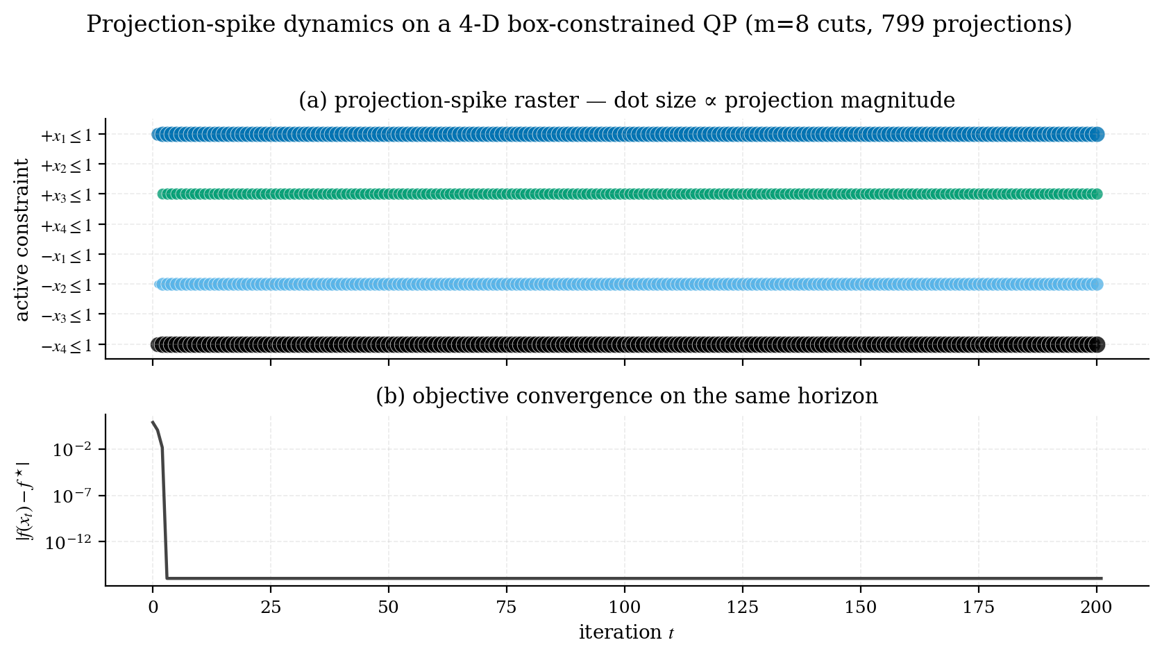
benchmarks/02_spike_raster.py on an 8-D QP over a 16-facet polytope.Each row is one inequality constraint . Each dot at column on row is a projection event: at iteration , constraint became active and the solver applied a spike to push back onto the feasible side. The dot’s size is proportional to the spike’s displacement norm : bigger dot, bigger correction. In the figure above the rows are coloured by whether they are still active at the true optimum, which is the distinction the raster is best at showing.
The bottom panel is the objective gap on the same iteration axis, so you can see which spikes happen at the high-energy phase versus the low-energy tail.
What you read off it
A few patterns to recognise:
Healthy convergence
Constraints recruited in turn and then firing steadily, with any early arrivals dropping out again. This is what the example above shows: one facet fires a short burst and falls silent, three more come in at iterations 21, 23 and 41 and then fire on every step. The steadily firing rows are the active set of the solution and the transients are the search that found it.
A non-convex or unbounded problem
Spikes that never settle down: the dot sizes don’t decrease and the active set keeps changing. Either the problem isn’t a QP (you’ve fed in a non-PSD Hessian), or your initialisation is sending the trajectory through a long sequence of facets.
A redundant constraint
A row that never fires. The constraint is in your formulation but is implied by other constraints. Worth removing to simplify the problem; sometimes it’s a bug (you intended that constraint to bind).
A poorly conditioned constraint
A row that fires every iteration with growing spike sizes. The auto step size is too aggressive for this constraint’s geometry. Drop k0_scale (default 0.5, try 0.2) and raise the iteration budget to match; see the accuracy figure on the home page for why the two have to move together.
Reproducing it on your own problem
SolverResult exposes the raw arrays:
result.spike_times          # iteration of each spike       shape (S,)
result.spike_constraints    # list of arrays of indices, one per spike
result.spike_norms          # ‖Δx‖_2 for each spike         shape (S,)
result.spike_deltas         # the Δx itself                 shape (S, n)
result.spike_violation_values  # the violation that triggered it
Since v0.5.0, bound constraints spike too, as implicit facets of the same sweep. Their IDs continue past the rows in a frozen order: lower facet i is reported as m + i and upper facet i as m + n + i, where m is the number of rows in C. Size your raster’s y-axis for m + 2n lanes if the problem has bounds, or those spikes will fall off the plot.
A minimal raster plot:
import matplotlib.pyplot as plt
import numpy as np

fig, ax = plt.subplots(figsize=(8, 3))
sizes = 6 + 70 * (result.spike_norms / result.spike_norms.max())
for k, (t, active) in enumerate(zip(result.spike_times, result.spike_constraints)):
    for j in active:
        ax.scatter([t], [j], s=[sizes[k]], color=f"C{j % 10}", alpha=0.8)

ax.set_xlabel("iteration")
ax.set_ylabel("constraint")
ax.set_yticks(np.arange(C.shape[0]))
ax.invert_yaxis()
plt.show()
The benchmark script benchmarks/02_spike_raster.py is the polished version, with an objective-gap subplot underneath and a consistent academic style.
Why this matters
Classical QP solvers give you the active set at the optimum. The spike raster gives you the active set as a time series: which constraints fought for influence and when, and which ones eventually won. This is the kind of insight that, in classical optimisation, lives only in textbooks. Here, it’s a built-in side effect of how the solver works.
Next
- Try running
example2_3d_polytope.pyand inspecting the resulting raster. A 3-D polytope with four constraints is the smallest interesting case. - Compare a healthy raster to one from a deliberately ill-conditioned problem (e.g. set
k0_scale=2.0and rerun a benchmark). See for yourself what “growing-amplitude spikes” looks like.