Curved walls spike too.

A force that would slip

A finger pushes on a surface. Coulomb friction says the tangential part of the contact force can be at most $\mu$ times the normal part, $\Vert f_t\Vert \le \mu f_n$: the force must stay inside a friction cone. Suppose a controller asks for a force $p$ outside that cone. It would slip. The solver’s job is to find the admissible force closest to $p$ (closest in the metric of the objective, a quadratic $\tfrac12 (f-p)^\top Q (f-p)$).

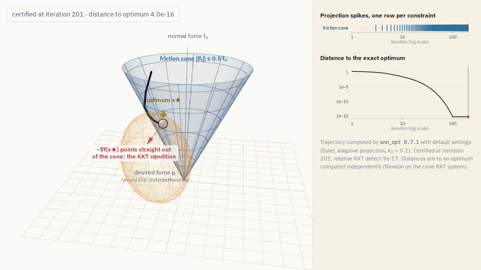
The state starts inside the cone and drifts toward $p$. After two clean drift steps, the third leaves the cone, and a spike projects it straight back onto the surface. From then on every step overshoots a little and is reset, so the state slides around the curved wall, spiking each step, until the drift pulls exactly along the cone’s outward normal. That is the optimum, and at the end you can see why: the orange level set of the objective just touches the cone there, and $-\nabla f(x^\star)$ points straight out of it. That is the KKT condition, $-\nabla f(x^\star) = \lambda\, \nabla g(x^\star)$ with $\lambda > 0$, drawn in three dimensions.

Two kinds of spike

A constraint now joins the sweep as a candidate, and a candidate can spike in one of two ways.

Cutters handle a differentiable convex inequality $g(x) \le 0$. The spike steps to the supporting halfspace at the current point,

$$x \;\leftarrow\; x - \frac{g(x)}{\Vert\nabla g(x)\Vert^2}\,\nabla g(x),$$

which is exactly the familiar row spike when $g$ is linear. Because $g$ is convex, the linearisation never cuts away a feasible point.

Exact projectors handle sets whose nearest point has a closed form. The spike is the reset $x \leftarrow P_K(x)$:

• a ball: scale back toward the centre;
• a second-order cone $\Vert z\Vert \le \mu t$: move to the nearest surface point, in the plane through the axis, $t' = (t + \mu\Vert z\Vert)/(1+\mu^2)$, $z' = \mu t'\, z/\Vert z\Vert$ (or the apex if the point is in the polar cone);
• the PSD cone: clip negative eigenvalues;
• a spectral-norm ball: clip singular values;
• an affine subspace $Bx = h$: the minimum-norm correction.

Every candidate competes in the same winner-take-all sweep as the rows, on one geometric scale: the most violated constraint, measured as a distance, fires first.

Why an exact projection gives an exact answer

Here is the fact that makes the conic extension more than a convenience. For a convex problem, $x^\star$ is optimal exactly when it is a fixed point of the projected-gradient map

$$T(x) = P_{\mathcal{F}}\big(x - \alpha\,\nabla f(x)\big), \qquad \text{for any } \alpha > 0.$$

So if a drift step followed by the spike sweep is the exact projection onto the feasible set, the dynamics stop exactly at the optimum, whatever the step size. The greedy row sweep achieves this when a single wall is active, which is why the solve on the home page ends $2\times10^{-16}$ from the optimum. At a vertex, where several walls are active together, the greedy sweep lands on a nearby feasible point instead, and that is the step-size-dependent offset described in the README’s accuracy section.

When sets meet: Dykstra’s algorithm

Projecting onto two sets one after the other finds a point in their intersection, but not the nearest one. Dykstra’s algorithm does find it, by remembering one correction per set between passes. snn_opt packages it as a single candidate, dykstra_projector, so a family of sets that are active together spikes as one exact projection.

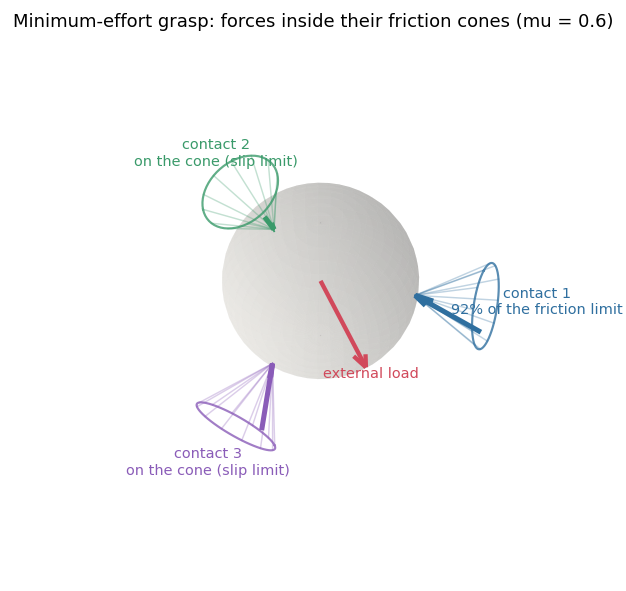
The worked example example8_friction_cone_grasp.py makes the difference concrete. With the equilibrium equations and the three cones wrapped in one Dykstra candidate, the solve certifies in 201 iterations and lands within $4\times10^{-13}$ of a Newton-polished reference. Hand the same four sets over separately and the sweep alternates between them: the run stops at its iteration cap with a relative KKT defect of $5\times10^{-2}$. The same trick fixes the vertex offset of ordinary linear constraints: joint_projector(C, d) projects all rows at once. On the 50-D benchmark problem of the README, with seven active rows, it takes the objective gap from the $6.7\times10^{-4}$ floor of the greedy sweep to $2.1\times10^{-10}$.

In code

import numpy as np
from snn_opt import OptimizationProblem, SNNSolver, SolverConfig, scaled_soc_projector

# Force f = (f_t1, f_t2, f_n) must satisfy ||(f_t1, f_t2)|| <= 0.5 * f_n.
cone = scaled_soc_projector(t_index=2, z_indices=[0, 1], mu=0.5)
p = np.array([1.53, -0.39, 1.29])                 # the force we would like

problem = OptimizationProblem(np.eye(3), -p,      # minimise 1/2 ||f - p||^2
                              np.zeros((0, 3)), np.zeros(0),
                              nonlinear_candidates=(cone,))
result = SNNSolver(problem, SolverConfig()).solve(np.array([0.0, 0.0, 1.0]))
print(result.final_x, result.converged)

Rows of C and candidates mix freely; a problem with no candidates runs exactly the polyhedral solver it always did.

How you know it is right

The KKT certificate behind converged=True extends to candidates: the fit adds each candidate’s normal cone to the constraint normals, including the whole polar cone at a nonsmooth point such as the apex. That is how the friction-cone solve above is certified.

Some problems get something stronger. When the objective is strongly convex and every candidate is an exact projector that the certificate can call (any set wrapped in dykstra_projector, the PSD cone, the spectral ball), the certificate becomes a direct bound on the error in the state itself,

$$\Vert x - x^\star\Vert \;\le\; \frac{\Vert x - T(x)\Vert}{\alpha\,\mu},$$

because $T$ is then a contraction. The grasp above is certified this way. (A Dykstra projector is trusted to its own inner tolerance, $10^{-12}$ relative to the size of the state by default; the bound does not charge for it.)

What runs where

Built-in sets (halfspaces, balls, second-order and friction cones, affine subspaces, and PSD or spectral-norm blocks up to 8×8) run on both the Python reference and the compiled C++ backend (backend='c'), kept in lockstep by parity tests. Custom cutters and projectors written as Python callbacks need backend='python'. On the hardware side, the newest Kria KV260 reference kernel performs ball and friction-cone resets natively on the FPGA datapath.

Next

• The full reference: docs/api.md.
• The derivation: docs/theory.md, §8.
• Hands-on: the friction-cone grasp tutorial.